Introduction
In this tutorial, we will describe how to use OneGenE-computed expansion lists to reconstruct a gene network, by means of the tools implemented in the OneGenExp website. As a case study, we will work on the stilbene synthases (STS) network. STSs catalyze the synthesis of resveratrol, the first step of the stilbenoid biosynthetic pathway. As a first step, their newtork will be computed and visualized, and then expanded to identify the genes directly connected to them. This analysis is described in the article “Vitis OneGenE, a causality-based approach to generate gene networks in Vitis vinifera, sheds light on the laccase and dirigent gene families”, submitted to Biomolecules Special Issue “Gene Regulatory Networks Controlling Secondary Metabolism in Plants: Computational Approaches and Mechanistic Insights”.
At the moment, we recommend using Firefox browser to do the network analyses, within which the ‘node label’ option works correctly.
-
Make a query with a list of grapevine genes
Go to the ‘OneGenE analysis’ page and follow the link, you will get to the query interface. Input the list of 45 STS genes using the 12X.V1 (the correspondence between the former V1 and the VCost.v3 annotations is available here) and click the ‘SEARCH’ button. NB: the query has a limit of 200 genes.
VIT_10s0042g00840,VIT_10s0042g00870,VIT_10s0042g00890,VIT_10s0042g00910,VIT_10s0042g00920,VIT_10s0042g00930,VIT_16s0100g00750,VIT_16s0100g00760,VIT_16s0100g00770,VIT_16s0100g00780,VIT_16s0100g00800,VIT_16s0100g00810,VIT_16s0100g00830,VIT_16s0100g00840,VIT_16s0100g00850,VIT_16s0100g00860,VIT_16s0100g00880,VIT_16s0100g00900,VIT_16s0100g00910,VIT_16s0100g00920,VIT_16s0100g00930,VIT_16s0100g00940,VIT_16s0100g00950,VIT_16s0100g00990,VIT_16s0100g01000,VIT_16s0100g01010,VIT_16s0100g01020,VIT_16s0100g01030,VIT_16s0100g01040,VIT_16s0100g01060,VIT_16s0100g01070,VIT_16s0100g01100,VIT_16s0100g01110,VIT_16s0100g01120,VIT_16s0100g01130,VIT_16s0100g01140,VIT_16s0100g01150,VIT_16s0100g01160,VIT_16s0100g01170,VIT_16s0100g01190,VIT_16s0100g01200
The user is now taken to the ‘Result’ page, which shows an overview of the OneGenE expansion lists in a table format. In the first column there is the ID of the expansion list, then the 12X.V1 ID (note that for clusters, the list of V1 IDs is truncated after the second ID, but upon clicking on the ‘?’ button or exporting the lists, all the IDs are indicated), the Functional annotation, Gene Name (when available) and the VCost.v3 ID.
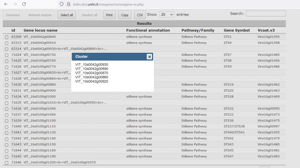
At this step, the user can select the genes of interest and download their expansion lists as a compressed file. Selecting at least two genes, the ‘Network analysis’ tab is activated and the user can do some gene network analyses, on a new page.
-
Building of the STS network
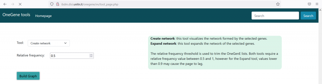
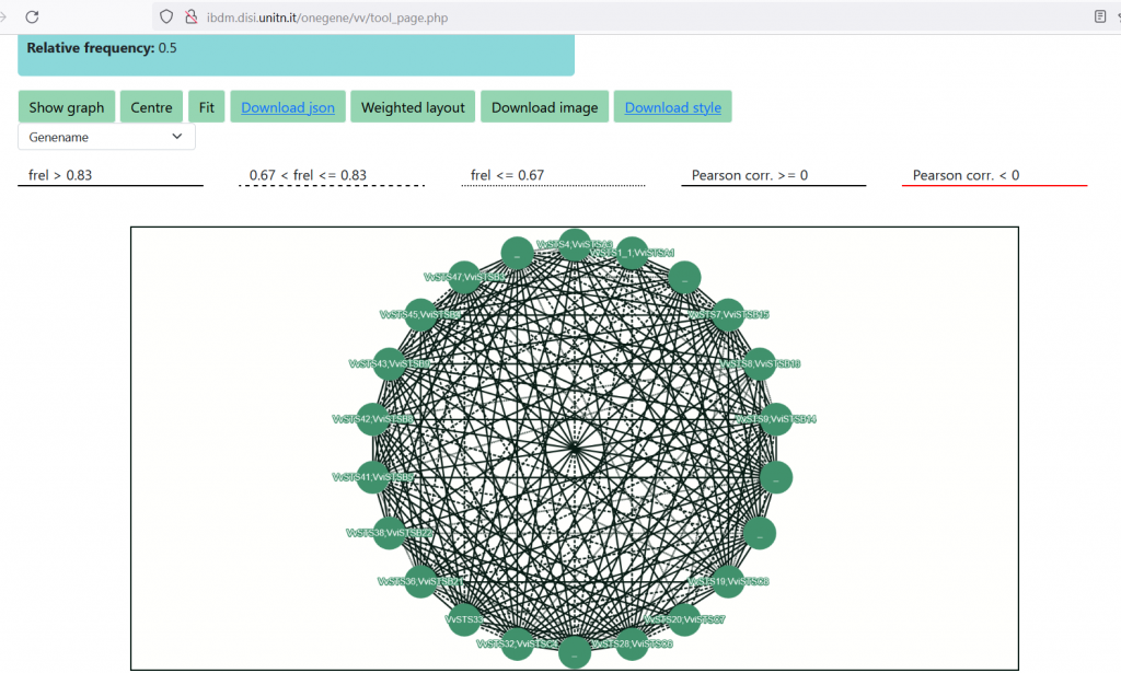
We can now visualize the interactions within the input STS genes as a graph, selecting the ‘Create Network’ tool and setting the Relative Frequency parameter. The latter, calculated as ‘F_rel= # times the gene is present in the output of the PC-algorithm / # times the gene is present in the input of the PC-algorithm’, has values between 0 and 1. However, only values between 0.5 and 1 are allowed, not to clog the system with too complex graphs. In this case, setting F_rel>=0.5, we trimmed the expansion lists at about 400 genes. Press the ‘Build’ button and wait, when the network is computed, press ‘Show Graph’ to visualize it. In the graph, STS genes are the nodes and the edges represent the reciprocal presence of geneA in geneB’s list and viceversa. Edges weight is computed as the mean of the F_rel values of the gene pair. Three line types (solid, dashed, dotted) are used to represent the strength of the interaction , while the color black or red represent positive or negative Pearson’s correlation values, as reported in the legend above the graph. The user can choose between three different types of node labeling (NB: it only works within Firefox, at the moment), which are the V1_ID, V3.VCost_ID and the gene symbol. The graph is interactive, as nodes can be manually moved; other layout options are available. By placing the cursor on a node, the adjacent nodes will be highlighted. The network can be downloaded as ‘.png’ image, or as a ‘.json’ file suitable for importing into Cytoscape for further user customization and analyses. To correctly interpret nodes and edges, please download the ‘Vitis_OneGenE_style.xlm‘ and import it into Cytoscape.
-
Expansion of the STS network
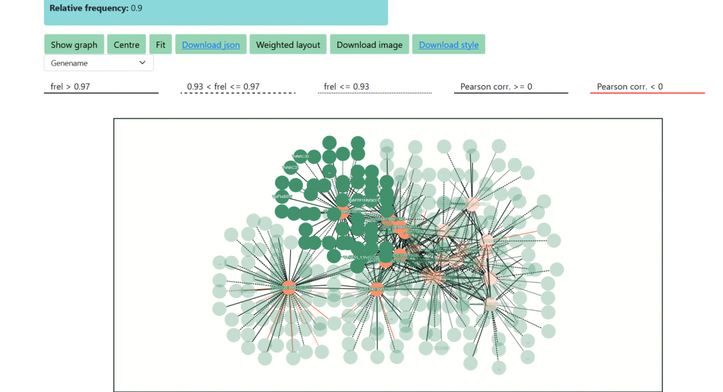
Another option is to identify the genes associated to the STS network. Selecting ‘Expand Network’ and setting the F_rel parameter to trim the lists, the list will be aggregated into one list. For the visualization, it is better to set high values, such as higher than 0.9; by setting lower values, the best option is to download the .json file and elaborate the network in Cytoscape.